Coherent Elastic Scattering

Coherent scattering is when periodic constructive growth or destructive cancellation of the scattered waves occur. This is a difficult phenomena to model, and thus LEAPR is currently limited to describing elastic coherent scattering for the following materials:

The differential coherent elastic scattering cross section is

\[\begin{split}\begin{gather} \sigma_{coh.el}(E,\mu)=\frac{\sigma_{coh}}{E}\sum_{E_i<E}f_i~\mathrm{e}^{-4W~E_i}~\delta(\mu-\mu_i)\\ \mu_i = 1-\frac{E_i}{E} \end{gather}\end{split}\]

and the integrated cross section (only energy dependence, integrated over angles), is

\[\sigma_{coh.el}(E)=\frac{\sigma_{coh}}{E}\sum_{E_i<E}f_i~\mathrm{e}^{-4W~E_i}.\]

where

• \(\sigma_{coh}\) is the effective bound coherent scattering cross section for the material

• \(W\) is the effective Debye Waller coefficient (defined using the phonon distribution \(\rho(\beta)\))

\[\begin{split}\begin{gather} W = \frac{\lambda}{Ak_bT}\\~\\ \lambda = \int_{-\infty}^\infty \frac{\rho(\beta)}{2\beta~\sinh(\beta/2)}~\mathrm{e}^{-\beta/2}~d\beta \end{gather}\end{split}\]

• \(E_i\) are the Bragg Edges

\[E_i = \frac{\hbar^2\tau_i^2}{8m}\]

• \(f_i\) are related to the crystallographic structure factors

Bragg Edges \(E_i\)

The Bragg edges are the locations in energy where the coherent elastic cross section will increase sharply. Recall the differential coherent scattering cross section,

\[\sigma_{coh.el}(E,\mu)=\frac{\sigma_c}{E}\sum_{E_i<E}f_i~\mathrm{e}^{-4W~E_i}~\delta(\mu-\mu_i).\]

It can be seen above that the coherent elastic cross section is zero below the first Bragg Edge (typicall 2-5 meV). It then jumps sharply to a value determined by \(f_1\) and the Debye-Waller factor \(W\). With increasing neutron energy \(E\), the cross section drops off as \(1/E\) until the second Bragg Edge is reached at \(E=E_2\). Again, the cross section jumps, and then resumes its \(1/E\) drop off. The size of the steps in the cross section gradually get smaller, until there is nothing left but the aymptotic \(1/E\) shape (which typically occurs near 1-2 eV). This behavior is also illustrated in the following plot for graphite:

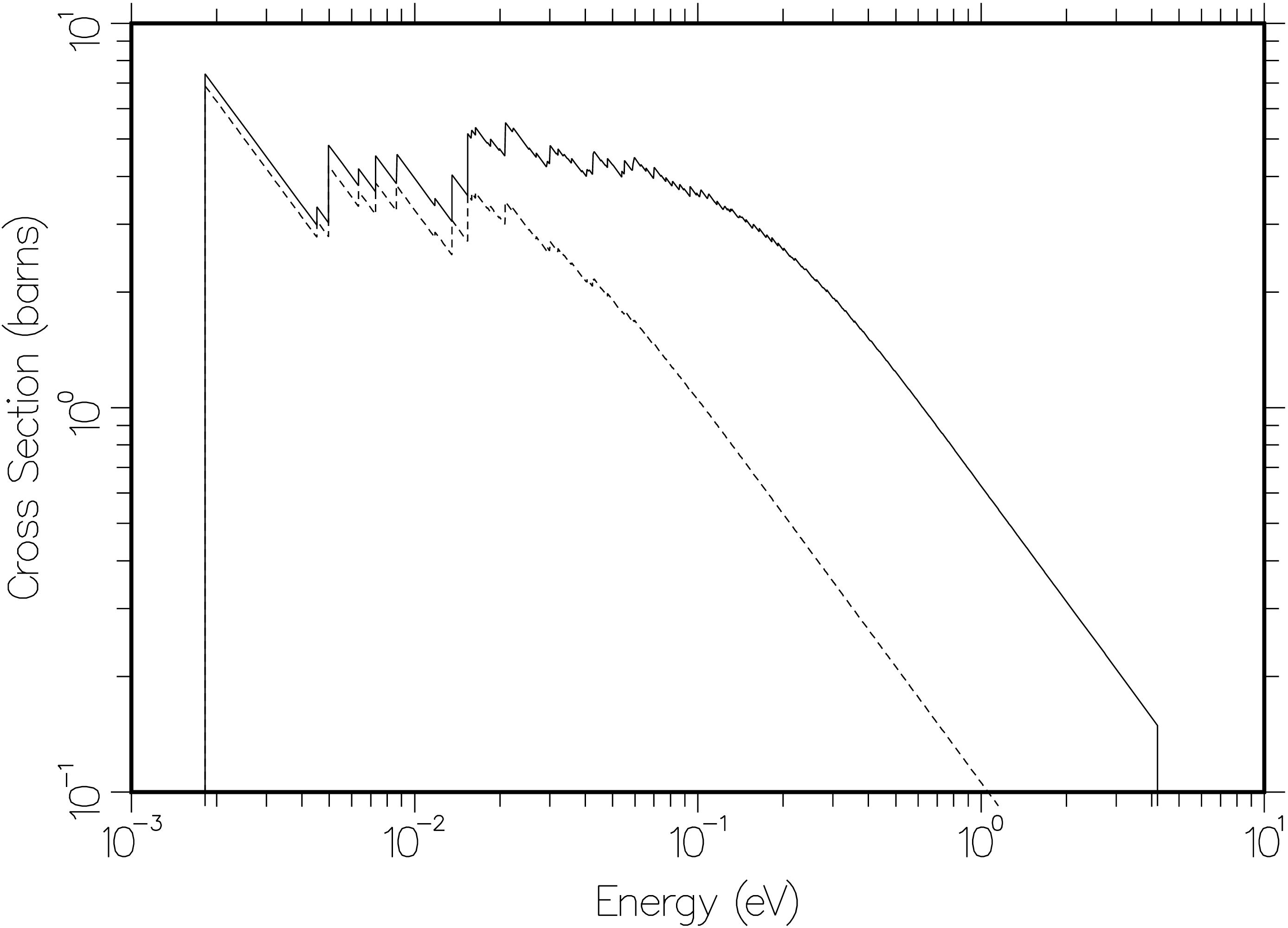
Fig. 2 The coherent elastic cross section for graphite at temperatures of 293.6K (solid) and 2000K (dashed) showing the Bragg peaks. Note that the 293.6K cross section near the 4 eV breakpoint is still an appreciable part of the 4.74 barn free cross section.

As mentioned above, the Bragg Edge locations \(E_i\) are

\[E_i = \frac{\hbar^2\tau_i^2}{8m}\]

where \(\tau_i\) are the length of the vectors in one particular “shell” of the reciprocal lattice, and \(m\) is the neutron mass.

\(f_i\) Factors

In the coherent elastic cross section sum, there are terms \(f_i\) that are defined as

\[f_i = \frac{2\pi\hbar^2}{4mNV}\sum_{\tau_i}\Big|F(\tau)\Big|^2\]

where the crystallographic stucture factor is

\[\Big|F(\tau)\Big|^2= \left|\sum_{j=1}^N\mathrm{e}^{i2\pi\phi_j}\right|\]

and \(N\) is the number of atoms in the unit cell, \(\phi_j=\vec{\tau}\cdot\vec{\rho_j}\) are the phases for the atoms, and \(\vec{\rho_j}\) are the atomic positions.

Multiple Atomic Species

Preparing coherent elastic scattering data for materials containing different atomic species (e.g., beryllium oxide) poses additional difficulties. For such materials, the bound coherent scattering cross section and Debye-Waller factor vary from nuclide to nuclide, thus for the \(j^{th}\) species are denoted as \(\sigma_j\) and \(W_j\), respectively. Recall that the coherent elastic scattering cross section is written as

\[\sigma_{coh.el}(E,\mu)=\frac{\sigma_c}{E}\sum_{E_i<E}f_i~\mathrm{e}^{-4W~E_i}~\delta(\mu-\mu_i)\]

where

\[f_i = \frac{2\pi\hbar^2}{4mNV}\sum_{\tau_i}\Big|F(\tau)\Big|^2.\]

Since the bound coherent scattering cross section an the Debye-Waller factor differ according to the species of atom, the differential scattering cross section is written as

\[\begin{split}\begin{align} \sigma_{coh.el}(E,\mu)&=\frac{\sigma_c}{E}\sum_{E_i<E}f_i~\mathrm{e}^{-4W~E_i}~\delta(\mu-\mu_i) \\ &=\frac{1}{E}\sum_{E_i<E}\left[\sigma_{coh}~f_i~\mathrm{e}^{-4WE_i}\right]\delta(\mu-\mu_i)\\ &=\frac{1}{E}\sum_{E_i<E}\left|\sum_{j=1}^N\sqrt{\sigma_j^{~}}~\mathrm{e}^{-2W_jE_i}~\mathrm{e}^{2i\pi\phi_j}\right|^2\delta(\mu-\mu_i) \end{align}\end{split}\]

\[\sigma_{coh}~\mathrm{e}^{-4WE_i}~f_i=\left|\sum_{j=1}^N\sqrt{\sigma_j^{~}}~\mathrm{e}^{-2W_jE_i}~\mathrm{e}^{2i\pi\phi_j}\right|^2\]

The effective bound coherent scattering cross section for these materials is given by

\[\sigma_{coh} = \sum_{j=1}^{N}\sigma_j\]

Since LEAPR and THERMR only work with one material at a time, they don’t have access to different values of \(W_j\) for the atoms in the unit cell. Therefore, they assume that \(W_jE_i\) is small (that \(W_j\) does not vary much from site to site). This allows us to simplify